LEO Pass Simulator: From State Error to Timing and Doppler Residual
A reproducible 600 km LEO-pass experiment that propagates epoch, satellite-state and UE-position errors into residual NR-NTN service-link timing and Doppler errors.
1. The engineering question
Release-17 NR-NTN relies on the UE’s position and the serving satellite’s ephemeris to update service-link timing and frequency pre-compensation. That creates a practical question:
For one declared LEO pass, how do errors in the satellite-state epoch, satellite position, satellite velocity and UE position translate into residual service-link timing and Doppler errors?
This page reports one controlled answer. It does not claim that the selected errors describe every deployed NTN system or that the results are universal 3GPP limits.
2. What makes the result reproducible
The complete artifact is public in the LEO Pass Simulator repository. The version reviewed for this page is commit 00fdabf.
It contains:
- the orbit, coordinate-frame, link-observable and error-injection source code;
- one complete JSON configuration;
- the full pass and signed residual time series as CSV;
- machine-readable summary and metadata files;
- regenerated SVG and PNG figures;
- 11 automated frame, orbit, numerical-consistency and artifact tests;
- a continuous-integration workflow; and
- an explicit validity boundary and extension plan.
Evidence boundary: this is a reproducible numerical experiment, not yet a high-fidelity orbit product or an original research claim. Its main value is that every reported number can be regenerated, inspected and challenged.
3. Declared baseline
The baseline models a circular ascending pass over Hyderabad:
| Parameter | Value |
|---|---|
| Observer | 17.385° N, 78.4867° E, 550 m |
| Epoch | 30 August 2026, 00:00:00 UTC |
| Circular-orbit altitude | 600 km |
| Inclination | 53° |
| Carrier frequency | 2.0 GHz |
| Elevation mask | 10° |
| Sampling interval | 1 s |
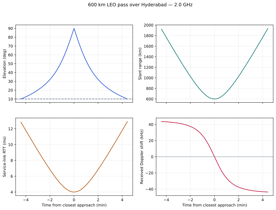
The orbit plane is constructed so that the satellite passes close to zenith at the declared epoch. Earth rotation is included in the ECI-to-ECEF transformation, and the stationary observer is placed using WGS-84 geodetic coordinates.
The reproduced pass has:
| Observable | Result |
|---|---|
| Visible duration above 10° | 530 s |
| Closest slant range | 600.000 km |
| Service-link RTT | 4.003–12.915 ms |
| Maximum absolute Doppler | 43.601 kHz |
| Maximum absolute Doppler rate | 535.937 Hz/s |
| Circular-orbit period | 96.659 min |
4. From orbit state to link observables
Let the satellite-to-UE relative position and velocity be
\[ \boldsymbol{\rho}=\mathbf r_s-\mathbf r_u, \qquad \mathbf v_r=\mathbf v_s-\mathbf v_u. \]
Slant range and line-of-sight range rate are
\[ \rho=|\boldsymbol{\rho}|, \qquad \dot{\rho}=\frac{\boldsymbol{\rho}}{\rho}\cdot\mathbf v_r. \]
The geometric service-link delay contribution is
\[ \tau_{\text{one-way}}=\frac{\rho}{c}, \qquad T_{\text{RTT}}=\frac{2\rho}{c}. \]
Using the received-minus-transmitted convention, first-order Doppler is
\[ f_D=-\frac{f_c}{c}\dot{\rho}. \]
The total orbital speed is not inserted directly into the Doppler equation. Only the velocity projected onto the instantaneous line of sight changes range. That is why Doppler reverses sign near closest approach even though the satellite remains fast.
5. Controlled error injections
Each estimated state is compared with the declared truth at every visible-pass sample:
| Scenario | Sweep | Injection |
|---|---|---|
| Epoch error | 1, 10, 100 ms | Evaluate the satellite at a shifted time and use that state at the true time |
| Satellite position error | 10, 100, 1000 m | Add an along-track ECEF position bias |
| Satellite velocity error | 0.01, 0.1, 1 m/s | Add an along-track ECEF velocity bias |
| UE position error | 1, 10, 100 m | Move the estimated stationary UE eastward |
Residual service-link RTT and Doppler are
\[ \Delta T_{\text{RTT}}=\frac{2(\hat{\rho}-\rho)}{c}, \qquad \Delta f_D=\hat f_D-f_D. \]
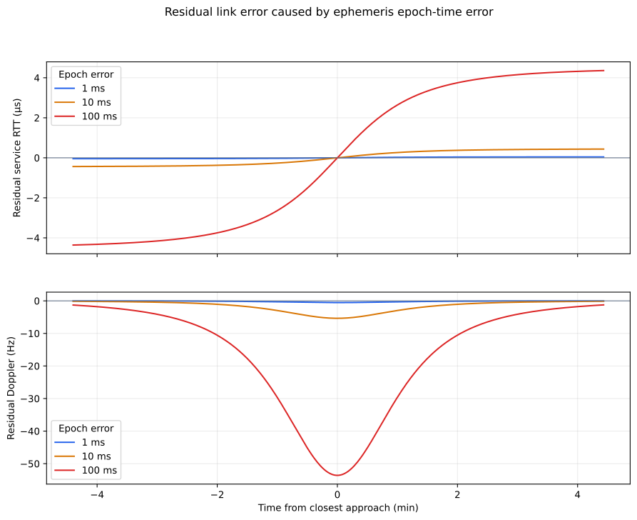
The full signed residuals are retained; the summary below reports maximum absolute values across the pass.
| Controlled error | Max residual service RTT | Max residual Doppler |
|---|---|---|
| Epoch +10 ms | 0.436 µs | 5.360 Hz |
| Satellite along-track position +100 m | 0.601 µs | 8.075 Hz |
| Satellite along-track velocity +0.1 m/s | 0 µs instantaneously | 0.601 Hz |
| UE position +10 m east | 0.039 µs | 0.476 Hz |
6. How to interpret the numbers
6.1 Epoch error becomes both position and velocity error
With a moving LEO satellite, evaluating the orbit at the wrong instant changes both predicted range and predicted range rate. In this small-error sweep, the response is almost linear: increasing the epoch error from 1 ms to 10 ms multiplies both maximum residuals by approximately ten.
6.2 Position and velocity errors affect different observables
The injected along-track position bias changes the instantaneous line of sight, so it changes both range and Doppler. The velocity-only experiment deliberately keeps the true position at the observation instant. Its instantaneous range—and therefore its instantaneous geometric delay—does not change, while its predicted range rate and Doppler do.
That zero timing result is a property of this specific instantaneous injection. If a velocity error were integrated forward as an orbit-state propagation error, it would accumulate into position and then timing error.
6.3 Geometry controls sensitivity
The maximum error does not have to occur at closest approach. Line-of-sight projection changes continuously across the pass, so an identical Cartesian state bias can have different range and range-rate effects at different elevations.
6.4 This is the service-link component
The reported RTT is the UE-to-payload service-link contribution. For a transparent NR-NTN system, the network-provided Common TA between the uplink synchronization reference point and the payload must be composed separately. Feeder-link Doppler and transponder frequency error are also outside this model.
7. Reproduce and inspect the experiment
git clone https://github.com/pppiyushh/leo-pass-simulator.git
cd leo-pass-simulator
python -m venv .venv
source .venv/bin/activate
python -m pip install -e .
leo-pass --config configs/hyderabad_600km.json \
  --output results/hyderabad_600km
python -m unittest discover -s tests -v
The repository commits the expected output beside the source. A reviewer can regenerate the study, compare the files, change one input and rerun the entire pass.
The automated checks cover:
- the J2000 GMST reference angle;
- ECI/ECEF position round trips;
- WGS-84 observer placement at the equator;
- circular-orbit radius, tangential velocity and period;
- ECEF velocity against a finite difference of position;
- closest-approach range and near-zenith elevation;
- Doppler sign reversal;
- small-error scaling; and
- successful CSV and SVG artifact generation.
8. Validity boundary
The first version intentionally uses an inspectable circular two-body model. It omits:
- J2, drag, maneuvers and other orbit perturbations;
- IERS Earth-orientation parameters, precession, nutation and polar motion;
- ionosphere, troposphere and atmospheric refraction;
- satellite, UE and network clock or oscillator error;
- feeder-link and transponder effects;
- SIB19 field encoding and quantization; and
- comparison with measured satellite data or a second propagator.
The next credibility step is therefore not to add more plots from the same model. It is to add a frozen TLE/SGP4 baseline or another independent implementation, quantify the difference, then study SIB19 quantization and Common-TA composition.
9. References and evidence
- Piyush Kumar Singh, LEO Pass Simulator v0.1.0, source, configuration, tests, data and figures.
- ETSI / 3GPP TS 38.300 V17.8.0, clauses 16.14.2.1–16.14.2.2, NR and NG-RAN overall description.
- National Geospatial-Intelligence Agency, Department of Defense World Geodetic System 1984.
- U.S. Naval Observatory, Computing approximate sidereal time.
- NASA, Basics of Space Flight: Gravity and Mechanics.